In this lab, we will use a diffraction grating to measure the wavelengths of the spectral lines emitted by a tube of atomic hydrogen. Using that information, we will measure the Rydberg constant.

• 1 Hydrogen Gas Tube (light source)
• 1 Diffraction Grating
• 1 Optical Bench (to hold diffraction grating)
• 1 Meter Stick
• 2 Mounted LEDs
• Record data in this Google Sheets data table

See KFJ Ch. 29 for the physics behind patterns of atomic spectra, and Ch. 17.3 for the physics behind diffraction gratings.

Specifically, there are two key equations we will be using in this lab.

First, the diffraction equation:

$$d\sin(\theta_m)=m\lambda$$

Second, the formula for the wavelength of light emitted in an atomic transition:

$$\frac{1}{\lambda_{n\rightarrow n'}}=R_H\left(\frac{1}{(n')^2}-\frac{1}{n^2}\right)$$

Here, we will be examining \(n'=2\) (the Balmer series).

Part I: Qualitative Observations

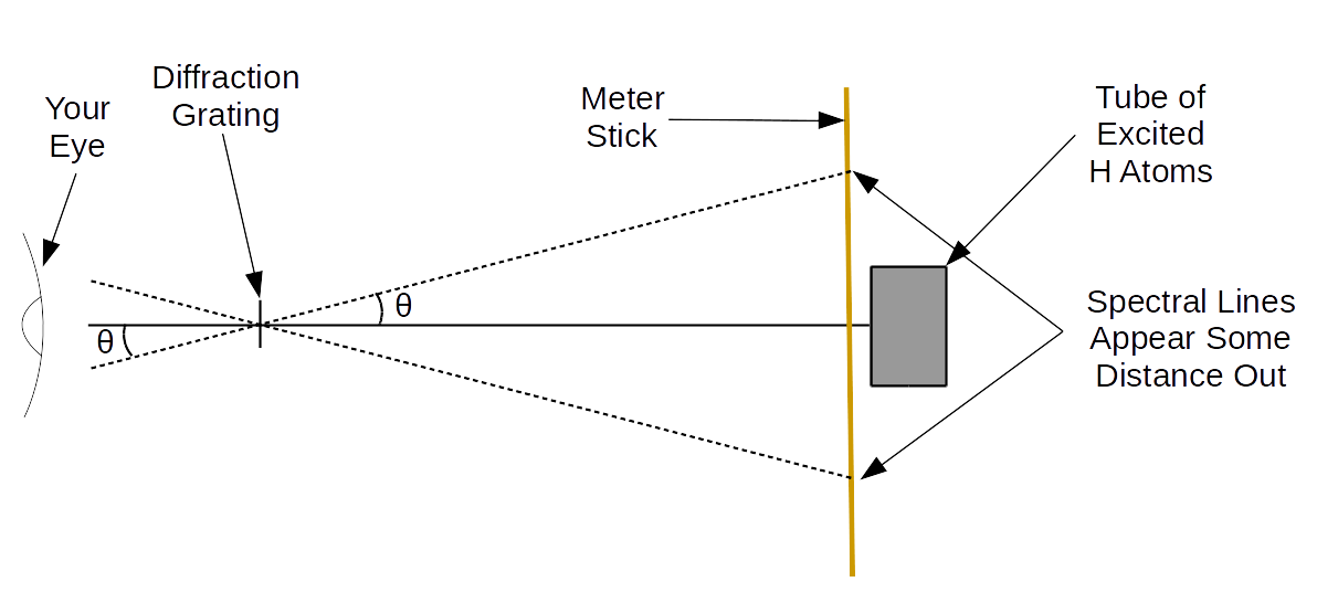
Set your diffraction grating ~\(40\)cm from the discharge tube. You should measure this distance with a meter stick, not read it off the optical bench, because there is extra distance between the end of the optical bench and the discharge tube.

Look through your grating and turn on the tube (and turn it off when not looking - you'll wear out the tube otherwise). You should observe one set of colored lines near the tube (three on either side). You should also observe a second, fainter set further out.

Potential difficulties:

• If you can't see the second spectral lines at all (and look carefully - they can be really faint), consult with your TA. They may be able to point out at least some of them. Placing the diffraction grating closer to the tube can help.
• If you see a green-yellow line, ignore it, as this results from external contamination.
• You may also observe a continuous spectrum between the spectral lines. This results from molecular hydrogen rather than atomic hydrogen (molecular spectral lines are closely-spaced, thus essentially continuous). While the electronics suffice to mostly excite the (naturally diatomic) hydrogen gas to its atomic state, some gas may remain.

Ideally, you want all six lines to be observable on each side (although one side is sufficient). Ensure that all lines you can see are "on the meter stick" (i.e., do not go beyond it on the opposite side). Sketch the spectrum you observe (qualitatively - exact numbers aren't required).

Record the location of the tube (on the meter stick) on your data sheet. Now, we want to (without moving the meter stick) record the location of the spectral lines.

Here, we will make use of the LEDs. Put one on the side of the stick on which you are measuring the spectral lines.

Turn it on and move it until it lines up with the line (as viewed through the diffraction grating), then use the indicator to read the position of the line. (It is probably best to have one partner will move the LEDs as the other partner looks through the grating and tells them where to move it.)

Record the positions of all six of the spectral lines on one side. Keep in mind that \(m=1\) is the inner set and \(m=2\) is the outer set.

On a sheet of graph paper, make a sketch of the spectral lines you observed. Mark which \(m\) the lines correspond to, and what color they are. You don't need to be quantitatively precise here - just a quick sketch of the general behavior of the lines.

Part II: Quantitative Observations

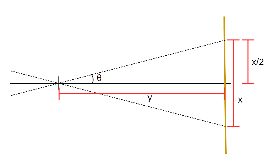
Now, move the grating farther away from the tube (~60cm away). Measure and record the actual distance between the tube and the grating, \(y\).

In this new arrangement, repeat the procedure from the previous part for measuring the spectral line positions, except this time, measure the \(m=1\) line positions on both the left and right sides. Estimate the uncertainty in these measurements.

Using that data and the knowledge that these diffraction gratings have \(\frac{1}{d}=500\) lines/mm, you should be able to deduce the wavelengths of the spectral lines. [Note: Some have \(13400\) lines/inch instead, but hopefully you won't be using those ones.]

First, as a preliminary step, from the knowledge of the lines/mm of the diffraction grating, calculate the distance between lines \(d\).

Note also that the red line is \(n=3\), the blue-green one is \(n=4\), and the purple one is \(n=5\).

Then, for each spectral line in part II, do the following:

• Calculate the separation distance \(x\) between the two \(m=1\) lines. Propagate uncertainties.
• Calculate the quantity \(x/2y\) and propagate uncertainty.
• Using trigonometry, calculate the angle \(\theta\) between the tube and the spectral line. This is the \(\theta_m\) (for \(m=1\)) that will go into the diffraction formula. You may find the following diagram helpful for this calculation (what is \(\tan(\theta)\)?):
  
• Using the diffraction formula, calculate the wavelength \(\lambda\) of the light. You can do uncertainty propagation in two ways here:
  • The technically-correct, fancy way: the Google Sheet will propagate your uncertainty from \(x/2y\) to \(\sin(\theta)\) automatically, through formulas that are beyond what you need to deal with. (If you know some calculus, Appendix A.3.1 of the Guide to Uncertainty Propagation & Error Analysis explains where these results come from.) From the uncertainty in \(\sin(\theta)\), calculate the uncertainty in \(\lambda\), assuming no uncertainty in \(d\).
  • The more approximate, simpler way: assume the relative error in \(x/2y\) is equal to the relative error in \(\lambda\). This is making a small angle approximation, essentially assuming \(\tan(\theta)\simeq\sin(\theta)\) for the purposes of error propagation.
• Calculate \(1/\lambda\). However you chose to calculate the uncertainty in \(\lambda\), propagate that uncertainty.
• Calculate the right-hand side of eq. 2 without the Rydberg constant; i.e., compute \(\frac{1}{4}-\frac{1}{n^2}\).

Finally, plot \(\frac{1}{\lambda}\) vs. \(\frac{1}{4}-\frac{1}{n^2}\). The slope of this plot will be the measurement of the Rydberg constant.

When you make this plot, for optimal results, do not include an intercept; do fit the line through the origin.

Analysis questions:

1. Qualitatively explain what you see in Part I using the diffraction formula.
2. Is your measurement of the Rydberg consistent with the theoretical value of \(1.097\times 10^7\)m\(^{-1}\)?
3. Why do we so strongly emphasize fitting the line through the origin in this lab, rather than running a general fit and letting the line naturally go through the origin? (Hint: this has to do with the number of degrees of freedom our data allows.)

Theoretical questions:

4. Why do we use \(n'=2\) in this lab? Why not \(n'=1\) or \(n'=3\)?

For further thought:

5. The spectrum described by the Rydberg formula results from taking a Coulomb attraction between an electron and a proton in quantum mechanics. However, there are actually corrections to the Hydrogen spectrum known as fine structure. Look into these corrections: what are the physical reasons behind them? (And why are they small?)
6. Smaller even than the above corrections, one finds hyperfine structure. What is the origin of these corrections? These corrections have a number of applications, including but not limited to:
   • Astronomy: One can locate hydrogen by looking at the very long-wavelength (radio) photons emitted by atoms transitioning between two states which differ in energy by a hyperfine correction. The wavelength of such photons is 21cm; thus, the spectral line is called the 21cm line.
   • SI Units: We use these corrections to create atomic clocks of very high precision, from which the second is defined (as exactly 9,192,631,770 times the period of a photon emitted in the hyperfine transition of Cs133).
   • Particle physics: We can make incredibly precise measurements of hyperfine transition frequencies. Being able to compute these frequencies to many decimal places and having these results be consistent with other experiments forms a high-precision test on our knowledge of particle physics.

Guide to Uncertainty Propagation & Error Analysis

Plotting Tool

Extra Atomic Spectrum Sketching Paper

Definition of a Second from NIST

Value of the Rydberg Constant from NIST

How CODATA determines the best value for Fundamental Constants